Chapter 1 Scientific modeling: abstract the complexity
Ce qui est simple est toujours faux. Ce qui ne l'est pas est inutilisable.
Paul Valéry (Mauvaises pensées et autres, 1942)
The notion of modeling is embedded in science, to the point that it has sometimes been used to define the very nature of scientific research. What is called a model can, however, correspond to very different realities which need to be defined before addressing the object of this thesis which will consist, if one wants to be mischievous, in analyzing models with other models. This semantic elucidation is all the more necessary as this thesis is interdisciplinary, suspended between systems biology and biostatistics. In order to convince the reader of the need for such a preamble, he is invited to ask a statistician and a biologist how they would define what a model is.
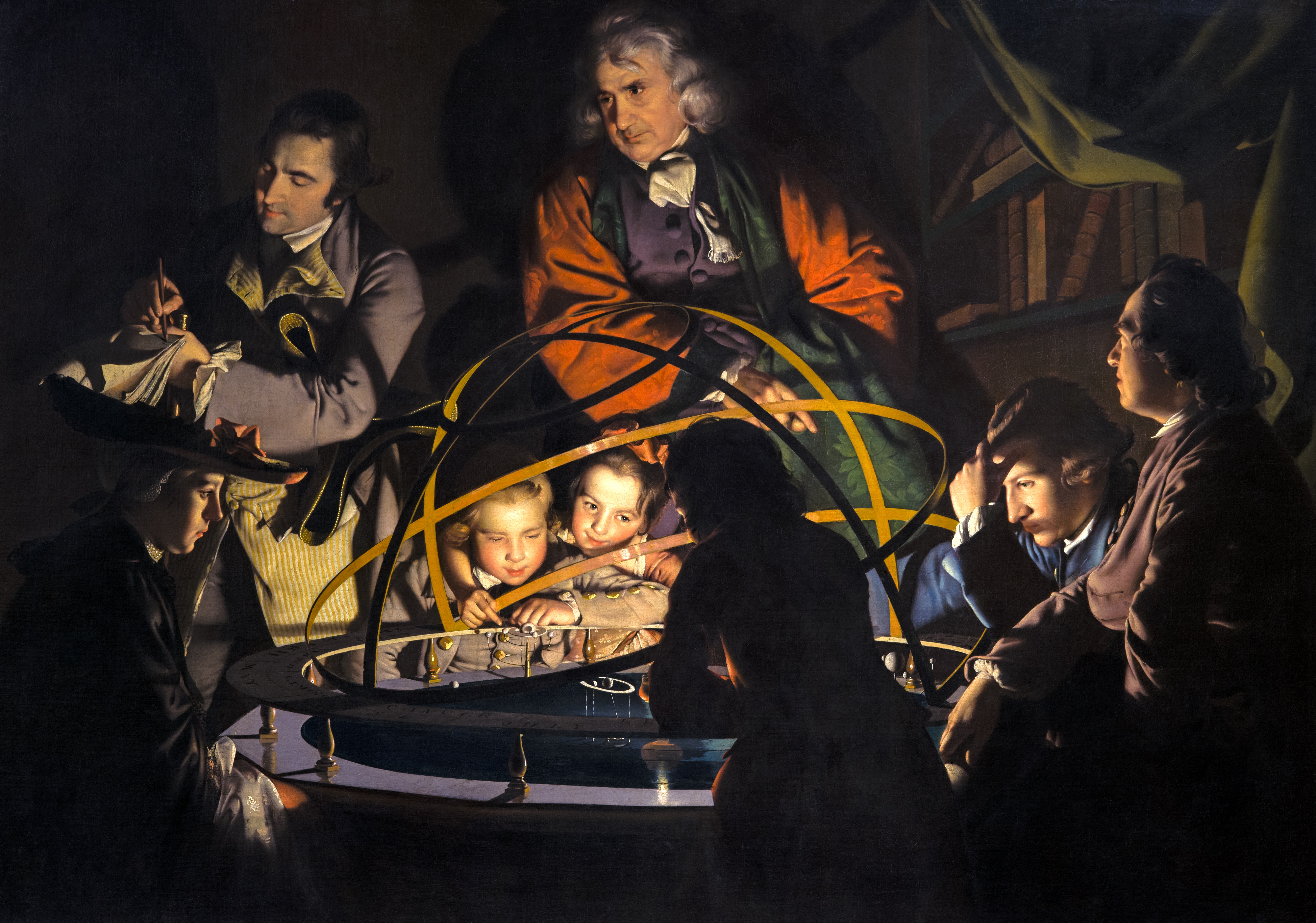
Figure 1.1: A scientist and his model. Joseph Wright of Derby, A Philosopher Giving a Lecture at the Orrery (in which a lamp is put in place of the sun), c. 1763-65, oil on canvas, Derby Museums and Art Gallery
1.1 What is a model?
1.1.1 In your own words
A model is first of all an ambiguous object and a polysemous word. It therefore seems necessary to start with a semantic study. Among the many meanings and synonymous proposed by the dictionary (Figure 1.2), while some definitions are more related to art, several find echoes in scientific practice. It is sometimes a question of the physical representation of an object, often on a reduced scale as in Figure 1.1, and sometimes of a theoretical description intended to facilitate the understanding of the way in which a system works (Collins 2020). It is even sometimes an ideal to be reached and therefore an ambitious prospect for an introduction.
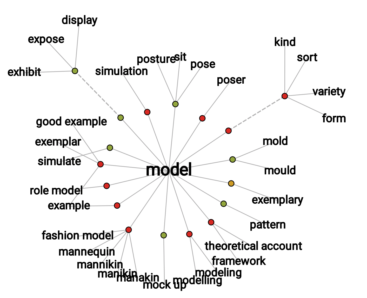
Figure 1.2: Network visualization of model thesaurus entries. Generated with the 'Visual Thesaurus' ressource
The narrower perspective of the scientist does not reduce the completeness of the dictionary's description to an unambiguous object (Bailer-Jones 2002). In an attempt to approach these multi-faceted objects that are the models, Daniela Bailer-Jones interviewed different scientists and asked them the same question: what is a model? Across the different profiles and fields of study, the answers vary but some patterns begin to emerge (Figure 1.3). A model must capture the essence of the phenomenon being studied. Because it eludes, voluntarily or not, many details or complexity, it is by nature a simplification of the phenomenon. These limitations may restrict its validity to certain cases or suspend it to the fulfilment of some hypotheses. They are not necessarily predictive, but they must be able to generate new hypotheses, be tested and possibly questioned. Finally, and fundamentally, they must provide insights about the object of study and contribute to its understanding.
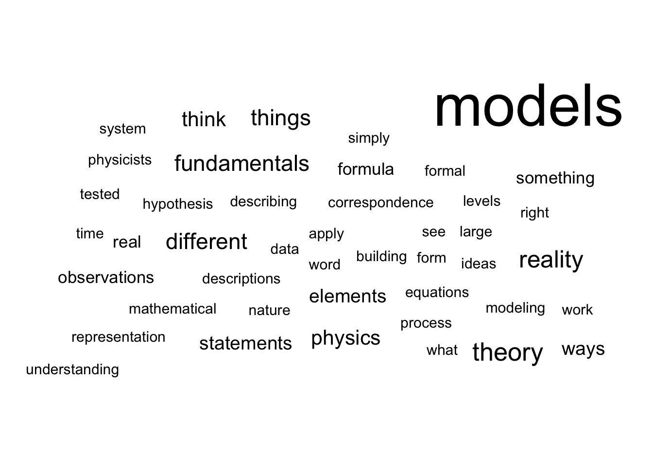
Figure 1.3: Scientists talk about their models: words cloud. Cloud of words summarizing the lexical fields used by scientists to talk about their models in dedicated interviews reported by Bailer-Jones (2002).
These definitions circumscribe the model object, its use and its objectives, but they do not in any way describe its nature. And for good reason, because even if we agree on the described contours, the biodiversity of the models remains overwhelming for taxonomists:
Probing models, phenomenological models, computational models, developmental models, explanatory models, impoverished models, testing models, idealized models, theoretical models, scale models, heuristic models, caricature models, exploratory models, didactic models, fantasy models, minimal models, toy models, imaginary models, mathematical models, mechanistic models, substitute models, iconic models, formal models, analogue models, and instrumental models are but some of the notions that are used to categorize models.
(Frigg and Hartmann 2020)
1.1.2 Physical world and world of ideas
Without claiming to be exhaustive, we can make a first simple dichotomy between physical/material and formal/intellectual models (Rosenblueth and Wiener 1945). The former consists in replacing the object of study by another object, just as physical but nevertheless simpler or better known. These may be models involving a change of scale such as the simple miniature replica placed in a wind tunnel, or the metal double helix model used by Watson and Crick to visualize DNA. In all these cases the model allows to visualize the object of study (Figure 1.4 A and B), to manipulate it and play with it to better understand or explain a phenomenon, just like the scientist with his orrery (Figure 1.1). In the case of biology, there are mainly model organisms such as drosophila, zebrafish or mice, for example. We then benefit from the relative simplicity of their genomes, a shorter time scale or ethical differences, usually to elucidate mechanisms of interest in humans. Correspondence between the target system and its model can sometimes be more conceptual, such as that ones relying on mechanical–electrical analogies: a mechanical system (e.g. a spring-mass system) can sometimes be represented by an electric network (e.g. a RLC circuit with a resistor, a capacitor and an inductor).
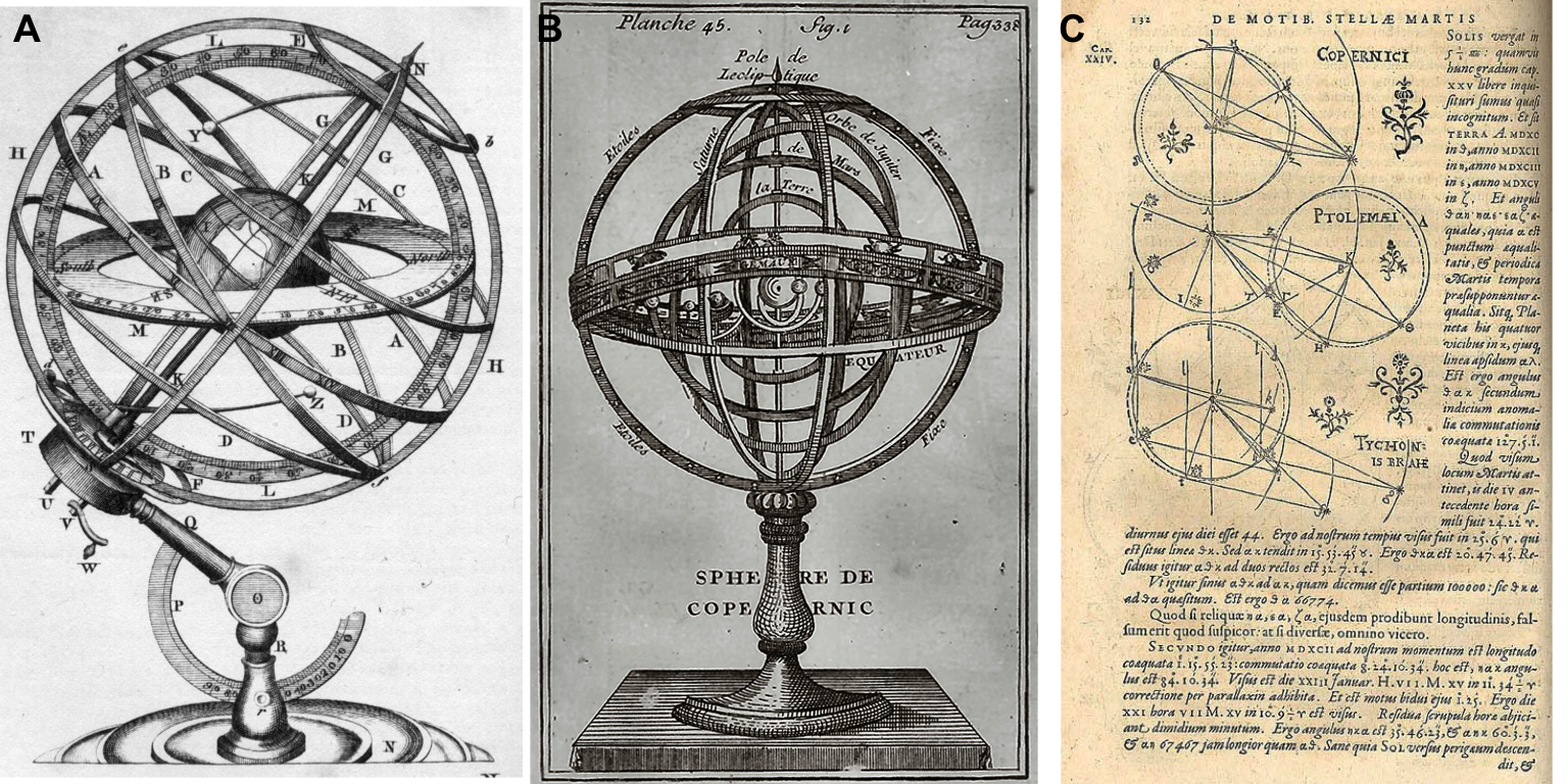
Figure 1.4: Orrery, planets and models. Physical models of planetary motion, either geocentric (Armillary sphere from Plate LXXVII in Encyclopedia Britannica, 1771) or heliocentric in panel B (Bion, 1751, catalogue Bnf) and some geometric representations by Johannes Kepler in panel C (in Astronomia Nova, 1609)
The model is then no longer simply a mimetic replica but is based on an intellectual equivalence: we are gradually moving into the realm of formal models (Rosenblueth and Wiener 1945). These are of a more symbolic nature and they represent the original system with a set of logical or mathematical terms, describing the main driving forces or similar structural properties as geometrical models of planetary motions summarized by Kepler in Figure 1.4C. Historically these models have often been expressed by sets of mathematical equations or relationships. Increasingly, these have been implemented by computer. Despite their sometimes less analytical and more numerical nature, many so-called computational models could also belong to this category of formal models. There are then many formalisms, discrete or continuous, deterministic or stochastic, based on differential equations or Boolean algebra (Fowler, Fowler, and Fowler 1997). Despite their more abstract nature, they offer similar scientific services: it is possible to play with their parameters, specifications or boundary conditions in order to better understand the phenomenon. One can also imagine these formal models from a different perspective, which starts from the data in a bottom-up approach instead of starting from the phenomenon in a top-down analysis. These models will then often be called statistical models or models of data (Frigg and Hartmann 2020). This distinction will be further clarified in section 1.2.
To summarize and continue a little longer with the astronomical metaphor, the study of a particularly complex system (the solar system) can be broken down into a variety of different models. Physical and mechanical models such as armillary spheres (1.4A and B) make it possible to touch the object of study. In addition, we can observe the evolution of models which, when confronted with data, have progressed from a geocentric to a heliocentric representation to get closer to the current state of knowledge. Sometimes, models with more formal representations are used to give substance to ideas and hypotheses (1.4C). One of the most conceptual forms is then the mathematical language and one can thus consider that the previously mentioned astronomical models find their culmination in Kepler's equations about orbits, areas and periods that describe the elliptical motion of the planets. We refer to them today as Kepler's laws. The model has become a law and therefore a paragon of mathematical modeling (Wan 2018).
1.1.3 Preview about cancer models
As we get closer to the subject of our study, and in order to illustrate these definitions more concretely, we can take an interest in the meaning of the word model in the context of cancer research. For this, we restrict our corpus to scientific articles found when searching for "cancer model" in the PubMed article database. Among these, we look at the occurrences of the word model and the sentences in which it is included. This cancer-related context of model is represented as a tree in Figure 1.5. Some of the distinctions already mentioned can be found here. The mouse and xenograft models, which will be discussed later in this thesis, represent some of the most common physical models in cancer studies. These are animal models in which the occurrence and mechanisms of cancer, usually induced by the biologist, are studied. On the other hand, prediction, prognostic or risk score models refer to formal models and borrow from statistical language.
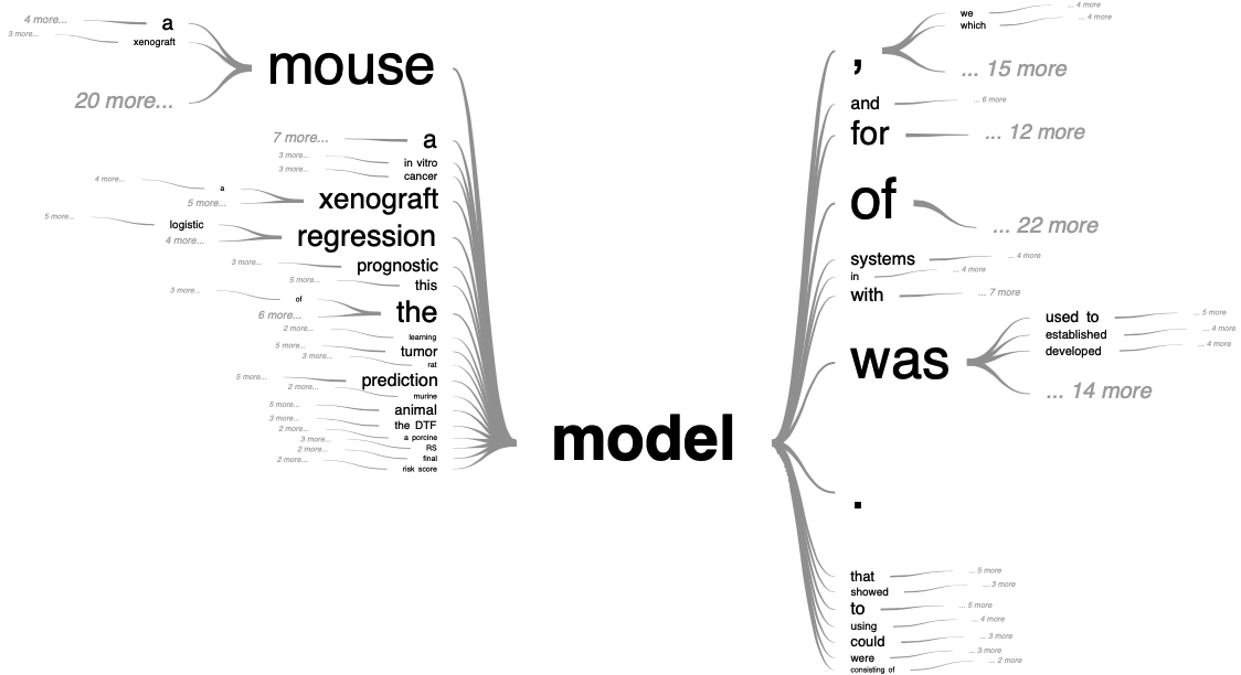
Figure 1.5: Tree visualization of model semantic context in cancer-related literature Generated with the 'PubTrees' tool by Ed Sperr, and based on most relevant PubMed entries for "cancer model" search.
Another way to classify cancer models may be to group them into the following categories: in vivo, in vitro and in silico. The first two clearly belong to the physical models but one uses whole living organisms (e.g. a human tumor implanted in an immunodeficient mouse) and the other separates the living from its organism in order to place it in a controlled environment (e.g. tumor cells in growth medium in a Petri dish). In the thesis, data from both in vivo and in vitro models will be used. However, unless otherwise stated, a model will always refer to a representation in silico. This third category, however, contains a very wide variety of models (Deisboeck et al. 2009), to which we will come back in chapter 3. A final ambiguity about the nature of the formal models used in this thesis needs to be clarified beforehand.
1.2 Statistics or mechanistic
A rather frequent metaphor is to compare formal models to black boxes that take in input \(X\) predictors, or independent variables, and output response variable(s) \(Y\), also named dependent variables. The models then split into two categories (Figure 1.6) depending on the answer to the question: are you modeling the inside of the box or not?
1.2.1 The inside of the box
The purpose of this section is to present in a schematic, and therefore somewhat caricatural, manner the two competing formal modeling approaches that will be used in this thesis and that we will call mechanistic modeling and statistical modeling. Assuming the unambiguous nature of the predictors and outputs we can imagine that the natural process consists in defining the result Y from the inputs X according to a function of a completely unknown form (Figure 1.6A).
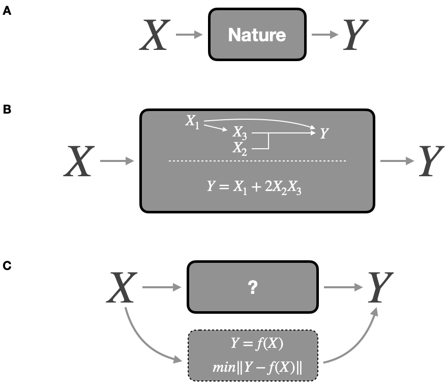
Figure 1.6: Different modeling strategies. (A) Data generation from predictors \(X\) to response \(Y\) in the natural phenomenon. (B) Mechanistic modeling defining mechanisms of data generation inside the box. (C) Statistical modeling finding the function \(f\) that gives the best predictions. Adapted from Breiman (2001b).
The first modeling approach, that we will call mechanistic, consists in building the box by imitating what we think is the process of data generation, or in other words, by representing the mechanisms at work (Figure 1.6B). This integration of prior knowledge can take different forms. In this thesis it will often come back to presupposing certain relations between entities according to what is known about their behaviour. \(X_1\) which acts on \(X_3\) may correspond to the action of one biological entity on another, supposedly unidirectional; just as the joint action of \(X_2\) and \(X_3\) may reflect a known synergy in the expression of genes or the action of proteins. Mathematically this is expressed here with a perfectly deterministic model defined a priori. All in all, in a purely mechanistic approach, the nature of the relations between entities should be linked to biological processes and the parameters in the model all have biological definitions in such a way that it could even be considered to measure them directly. For example, the coefficient \(2\) multiplying \(X_2X_3\) can correspond to a stoichiometric coefficient or a reaction constant which have a theoretical justification or are accessible by experimentation. In some fields of literature these models are sometimes called mathematical models because they propose a mathematical translation of a phenomenon, which does not start from the data in a bottom-up approach but rather from a top-down theoretical framework. In this thesis we will adhere to the mechanistic model name, which is more transparent and less ambiguous compared to other approaches also based on mathematics, without necessarily the other characteristics described above.
The second approach, often called statistical modeling, or sometimes machine learning depending on the precise context and objective, does not necessarily seek to reproduce the natural process of data generation but to find the function allowing the best prediction of \(Y\) from \(X\) (Figure 1.6C). Pushed to the limit, they are an "idealized version of the data we gain from immediate observation" (Frigg and Hartmann 2020), thus providing a phenomenological description. The methods and algorithms used are then intended to be sufficiently flexible and to make the fewest possible assumptions about the relationships between variables or the distribution of data. Without listing them exhaustively, the approaches such as simple linear regressions or more complex support vector machines (Cortes and Vapnik 1995) or random forests (Breiman 2001a), which will sometimes be mentioned in this thesis, fall into this category which contains many others (Hastie, Tibshirani, and Friedman 2009).
Several discrepancies result from this difference in nature between mechanistic and statistical models, some of which are summarized in the Table 1.1. In a somewhat schematic way, we can say that the mechanistic model first asks the question of how and then looks at the result for the output. Conversely, the statistical model first tries to approach the Y and then possibly analyses what can be deduced from it, regarding the importance of the variables or their relationships in a post hoc approach (Ishwaran 2007; Manica et al. 2019). The greater flexibility of statistical methods makes it possible to better accept the heterogeneity of the variables, but this is generally done at the cost of a larger number of parameters and therefore requires more data. Moreover, statistical models can be considered as inductive, since they are able to use already generated data to identify patterns in it. Conversely, mechanistic models are more deductive and they can theoretically allow to extrapolate beyond the original data or knowledge used to build the model (Baker et al. 2018). Finally, the most relevant way of assessing the value or adequacy of these models may be quite different. A statistical model is measured by its ability to predict output in a validation dataset different from the one used to train its parameters. The mechanistic model will also be evaluated on its capacity to approach the data but also to order it, to give a meaning. If its pure predictive performance is generally inferior, how can the value of understanding be assessed? This question will be one of the threads of the dissertation.
| Mechanistic modeling | Statistical modeling |
|---|---|
| Definition | |
| Seeks to establish a mechanistic relationship between inputs and outputs | Seeks to establish statistical relationships between inputs and outputs |
| Pros and cons | |
| Presupposes and investigates causal links between the variables | Looks for patterns and establishes correlations between variables |
| Capable of handling small datasets | Requires large datasets |
| Once validated, can be used as a predictive tool in new situations possibly difficult to access through experimentation | Can only make predictions that relate to patterns within the data supplied |
| Difficult to accurately incorporate information from multiple space and time scales due to constrained specifications | Can tackle problems with multiple space and time scales thanks to flexible specifications |
| Evaluated on closeness to data and ability to make sense of it | Evaluated based on predictive performance |
Mechanistic and statistical models are not perfectly exclusive and rather form the two ends of a spectrum. The definitions and classification of some examples is therefore still partly personal and arbitrary. For instance, the example in 1.6B can be transformed into a model with a more ambiguous status:
\[logit(P[Y=1])=\beta_1X_1 + \beta_{23}X_2X_3\]
This model is deliberately ambiguous. As a logistic model, it is therefore naturally defined as a statistical model. But the definition of the interaction between \(X_2\) and \(X_3\) denotes a mechanistic presupposition. The very choice of a logistic and therefore parametric model could also result from a knowledge of the phenomenon, even if in practice it is often a default choice for a binary output. Finally, the nature of the parameters \(\beta_{1}\) and \(\beta_{23}\) is likely to change the interpretation of the model. If they are deduced from the data and therefore optimized to fit Y as well as possible, one will think of a statistical model whose specification is nevertheless based on knowledge of the phenomenon. On the other hand, one could imagine that these parameters are taken from the biochemistry literature or other data. The model will then be more mechanistic. The boundary between these models is further blurred by the different possibilities of combining these approaches and making them complementary (Baker et al. 2018; Salvucci, Rahman, et al. 2019).
1.2.2 A tale of prey and predators
The following is a final general illustration of the concepts and procedures introduced with respect to statistical and mechanistic models through a famous and characteristic example: the Lotka-Volterra model of interactions between prey and predators. This model was, like many students, my first encounter with what could be called mathematical biology. The Italian mathematician Vito Volterra states this system for the first time studying the unexpected characteristics of fish populations in the Adriatic Sea after the First World War. Interestingly, Alfred Lotka, an American physicist deduced the exact same system independantly, starting from very generic process of redistribution of matter among the several components derived from law of mass action (Knuuttila and Loettgers 2017). A detailed description of their works and historical formulation can be found in original articles (Lotka 1925; Volterra 1926) or dedicated reviews (Knuuttila and Loettgers 2017).
The general objective is to understand the evolution of the populations of a species of prey and its predator, reasonably isolated from outside intervention. Here we will use Canada lynx (Lynx canadensis) and snowshow hare (Lepus americanus) populations for which an illustrative data set exists (Hewitt 1917). In fact, commercial records listing the quantities of furs sold by trappers to the Canadian Hudson Bay Company may represent a proxy for the populations of these two species as represented in Figure 1.7A. Denoting the population of lynx \(L(t)\) and the population of hare \(H(t)\) it can be hypothesized that prey, in the absence of predators, would increase in population, while predators on their own would decline in the absence of prey. A prey/predator interaction term can then be added, which will positively impact predators and negatively impact prey. The system can then be formalized with the following differential questions with all coefficients \(a_1, a_2, b_1, b_2 >0\):
\[\dfrac{dH}{dt}=a_1H-a_2HL\]
\[\dfrac{dL}{dt}=-b_1L+b_2HL\]
\(a_1H\) represents the growth rate of the hare population (prey), i.e., the population grows in proportion to the population itself according to usual birth modeling. The main losses of hares are due to predation by lynx, as represented with a negative coefficient in the \(-a_2HT\) term. It is therefore assumed that a fixed percentage of prey-predator encounters will result in the death of the prey. Conversely, it is assumed that the growth of the lynx population depends primarily on the availability of food for all lynxes, summarized in the \(b_2HL\) term. In the absence of hares, the lynx population decreases, as denoted by the coefficient \(-b_1L\). Important features of mechanistic models are illustrated here: the equations are based on a priori knowledge or assumptions about the structure of the problem and the parameters of the model can be interpreted. \(a_1\), for example, could correspond to the frequency of litters among hares and the number of offspring per litter.
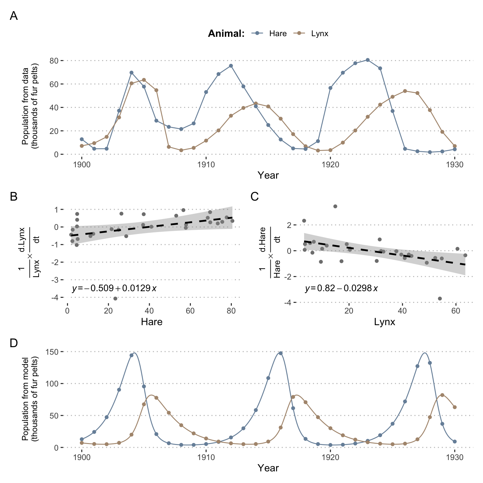
Figure 1.7: Some analyses around Lotka-Volterra model of a prey-predator system. (A) Evolution of lynx and hares populations based on Hudson Bay Company data about fur pelts. (B) and (C) Linear regression for estimation of parameters. (D) Evolution of lynx and hare populations as predicted by the model based on inferred parameters and initial conditions.
This being said, the structure of the model having been defined a priori, it remains to determine its parameters. Two options would theoretically be possible: to propose values based on the interpretation of the parameters and ecological knowledge, or to fit the model to the data in order to find the best parameters. For the sake of simplicity, and because this example has only a pedagogical value in this presentation, we propose to determine them approximately using the following Taylor-based approximation:
\[\dfrac{1}{y(t)} \dfrac{dy}{dt} \simeq \dfrac{1}{y(t)} \dfrac{y(t+1)-y(t-1)}{2}\]
By applying this approximation to the two equations of the differential system and plotting the corresponding linear regressions (Figures 1.7B and C), we can obtain an evaluation of the parameters such as \(a_1=0.82\), \(a_2=0.0298\), \(b_1=0.509\), \(b_2=0.0129\). By matching the initial conditions to the data, the differential system can then be fully determined and solved numerically (Figures 1.7D). Comparison of data and modeling provides a good illustration of the virtues and weaknesses of a mechanistic model. Firstly, based on explicit and interpretable hypotheses, the model was able to recover the cyclical behaviour and dependencies between the two species: the increase in the lynx population always seems to be preceded by the increase in the hare population. However, the amplitude of the oscillations and their periods are not exactly those observed in the data. This may be related to approximations in the evaluation of parameters, random variation in the data or, of course, simplifications or errors in the structure of the model itself.
Besides, if one tries to carry out a statistical modeling of these data, it is very likely that it is possible to approach the curve of populations evolution much closer, especially for the hares. But should it be expressed simply as a function of time or should a joint modeling be proposed? The nature of the causal link between prey and predators will be extremely difficult to establish without strong hypotheses such as those of the mechanistic model. On the other hand, if populations in later years had to be predicted as accurately as possible, it is likely that a sufficiently well-trained statistical model would perform better. Finally, and this is a fundamental difference, the mechanistic model enables to test cases or hypotheses that go beyond the scope of the data. Quite simply, by playing with the variables or parameters of the model, we can predict the exponential decrease of predators in the absence of prey and the exponential growth of prey in the absence of predator. More generally, it is also possible to study analytically or numerically the bifurcation points of the system in order to determine the families of behaviours according to the relative values of the parameters (Flake 1998). It is not possible to infer these new or hypothetical behaviours directly from the data of the statistical model. This is theoretically possible on the basis of the mechanistic model, provided that it is sufficiently relevant and that its operating hypotheses cover the cases under investigation. Now that the value of mechanistic models has been illustrated in a fairly theoretical example, all that remains is to explore in the next chapters how they can be built and used in the context of cancer.
1.3 Simplicity is the ultimate sophistication
Before concluding this modeling introduction, it is important to highlight one of the most important points already introduced in a concise manner by the poet Paul Valéry at the beginning of this chapter. Whatever its nature, a model is always a simplified representation of reality and by extension is always wrong to a certain extent. This is a generally well-accepted fact, but it is crucial to understand the implications for the modeler. This simplification is not a collateral effect but an intrinsic feature of any model:
No substantial part of the universe is so simple that it can be grasped and controlled without abstraction. Abstraction consists in replacing the part of the universe under consideration by a model of similar but simpler structure. Models, formal and intellectual on the one hand, or material on the other, are thus a central necessity of scientific procedure.
(Rosenblueth and Wiener 1945)
Therefore, a model exists only because we are not able to deal directly with the phenomenon and simplification is a necessity to make it more tractable (Potochnik 2017). This simplification appeared many times in the studies of frictionless planes or theoretically isolated systems, in a totally deliberate strategy. However, this idealization can be viewed in several ways (Weisberg 2007). One of them, called Aristotelian or minimal idealization, is to eliminate all the properties of an object that we think are not relevant to the problem in question. This amounts to lying by omission or making assumptions of insignificance by focusing on key causal factors only (Frigg and Hartmann 2020). We therefore refer to the a priori idea that we have of the phenomenon. The other idealization, called Galilean, is to deliberately distort the theory to make it tractable as explicited by Galileo himself:
We are trying to investigate what would happen to moveables very diverse in weight, in a medium quite devoid of resistance, so that the whole difference of speed existing between these moveables would have to be referred to inequality of weight alone. Since we lack such a space, let us (instead) observe what happens in the thinnest and least resistant media, comparing this with what happens in others less thin and more resistant.
This fairly pragmatic approach should make it possible to evolve iteratively, reducing distortions as and when possible. This could involve the addition of other species or human intervention into the Lotka-Volterra system described above. A three-species Lotka-Volterra model can however become chaotic (Flake 1998), and therefore extremely difficult to use and interpret, thus underlining the importance of simplifying the model.
We will have the opportunity to come back to the idealizations made in the course of the cancer models but it is already possible to give some orientations. The biologist who seeks to study cancer using cell lines or animal models is clearly part of Galileo's lineage. The mathematical or in silico modeler has a more balanced profile. The design of qualitative mechanistic models based on prior knowledge, which is the core of the second part of the thesis, is more akin to minimal idealization, which seeks to highlight the salient features of a system. The Galilean consistins in studying mathematically tractable systems was also important. To take the example of prey-predator interactions, a differential system with more variables quickly becomes impossible to solve by hand. The development of more and more powerful computers has apparently pushed back the limits of the computationally tractable systems and thus of Galilean idealization. However, this is always necessary, for example in high-dimensional statistical approaches (thousands of variables) where the modelers decide to consider the variables independently while neglecting their interactions.
Because of the complexity of the phenomena, simplification is therefore a necessity. The objective then should not necessarily be to make the model more complex, but to match its level of simplification with its assumptions and objectives. Faced with the temptation of the author of the model, or his reviewer, to always extend and complicate the model, it could be replied with Lewis Carrol words3:
"That’s another thing we’ve learned from your Nation," said Mein Herr, "map-making. But we’ve carried it much further than you. What do you consider the largest map that would be really useful?"
"About six inches to the mile."
"Only six inches!" exclaimed Mein Herr. "We very soon got to six yards to the mile. Then we tried a hundred yards to the mile. And then came the grandest idea of all! We actually made a map of the country, on the scale of a mile to the mile!"
"Have you used it much?" I enquired.
"It has never been spread out, yet," said Mein Herr: "the farmers objected: they said it would cover the whole country, and shut out the sunlight! So we now use the country itself, as its own map, and I assure you it does nearly as well."
Lewis Carroll, Sylvie and Bruno (1893)
Summary
Any scientific model has the vocation to allow the understanding of its object of study by proposing a simplification simpler to handle. A model can be physical or purely intellectual. This thesis will focus on the latter, in particular models that explicitly highlight the mechanisms and relationships between the underlying entities of the system. These models will be called mechanistic and sometimes opposed to statistical models or machine learning models which do not presuppose a priori knowledge on the internal mechanisms of the system.
References
Bailer-Jones, Daniela M. 2002. “Scientists’ Thoughts on Scientific Models.” Perspectives on Science 10 (3). MIT Press: 275–301.
Baker, Ruth E, Jose-Maria Pena, Jayaratnam Jayamohan, and Antoine Jérusalem. 2018. “Mechanistic Models Versus Machine Learning, a Fight Worth Fighting for the Biological Community?” Biology Letters 14 (5). The Royal Society: 20170660.
Breiman, Leo. 2001a. “Random Forests.” Machine Learning 45 (1). Springer: 5–32.
Breiman, Leo. 2001b. “Statistical Modeling: The Two Cultures (with Comments and a Rejoinder by the Author).” Statistical Science 16 (3). Institute of Mathematical Statistics: 199–231.
Collins. 2020. The Collins English Dictionary. HarperCollins.
Cortes, Corinna, and Vladimir Vapnik. 1995. “Support-Vector Networks.” Machine Learning 20 (3). Springer: 273–97.
Deisboeck, Thomas S, Le Zhang, Jeongah Yoon, and Jose Costa. 2009. “In Silico Cancer Modeling: Is It Ready for Prime Time?” Nature Clinical Practice Oncology 6 (1). Nature Publishing Group: 34–42.
Flake, Gary William. 1998. The Computational Beauty of Nature: Computer Explorations of Fractals, Chaos, Complex Systems, and Adaptation. MIT press.
Fowler, Andrew Cadle, Anna C Fowler, and AC Fowler. 1997. Mathematical Models in the Applied Sciences. Vol. 17. Cambridge University Press.
Frigg, Roman, and Stephan Hartmann. 2020. “Models in Science.” In The Stanford Encyclopedia of Philosophy, edited by Edward N. Zalta, Spring 2020. https://plato.stanford.edu/archives/spr2020/entries/models-science/; Metaphysics Research Lab, Stanford University.
Hastie, Trevor, Robert Tibshirani, and Jerome Friedman. 2009. The Elements of Statistical Learning: Data Mining, Inference, and Prediction. Springer Science & Business Media.
Hewitt, C Gordon. 1917. “Conservation of Wild Life in Canada.” Nature Publishing Group.
Ishwaran, Hemant. 2007. “Variable Importance in Binary Regression Trees and Forests.” Electronic Journal of Statistics 1. The Institute of Mathematical Statistics; the Bernoulli Society: 519–37.
Knuuttila, Tarja, and Andrea Loettgers. 2017. “Modelling as Indirect Representation? The Lotka–Volterra Model Revisited.” The British Journal for the Philosophy of Science 68 (4). Oxford University Press: 1007–36.
Lotka, AJ. 1925. “Principles of Physical Biology.” Baltimore: Waverly.
Manica, Matteo, Ali Oskooei, Jannis Born, Vigneshwari Subramanian, Julio Sáez-Rodríguez, and María Rodríguez Martínez. 2019. “Toward Explainable Anticancer Compound Sensitivity Prediction via Multimodal Attention-Based Convolutional Encoders.” Molecular Pharmaceutics. ACS Publications.
Potochnik, Angela. 2017. Idealization and the Aims of Science. University of Chicago Press.
Rosenblueth, Arturo, and Norbert Wiener. 1945. “The Role of Models in Science.” Philosophy of Science 12 (4). Williams; Wilkins Co.: 316–21.
Salvucci, Manuela, Arman Rahman, Alexa J Resler, Girish M Udupi, Deborah A McNamara, Elaine W Kay, Pierre Laurent-Puig, et al. 2019. “A Machine Learning Platform to Optimize the Translation of Personalized Network Models to the Clinic.” JCO Clinical Cancer Informatics 3. American Society of Clinical Oncology: 1–17.
Volterra, Vito. 1926. “Fluctuations in the Abundance of a Species Considered Mathematically.” Nature Publishing Group.
Wan, Frederick YM. 2018. Mathematical Models and Their Analysis. Vol. 79. SIAM.
Weisberg, Michael. 2007. “Three Kinds of Idealization.” The Journal of Philosophy 104 (12): 639–59.