Chapter 8 Clinical evidence generation and causal inference

Maudit
soit le père de l'épouse
du forgeron qui forgea le fer de la cognée
avec laquelle le bûcheron abattit le chêne
dans lequel on sculpta le lit
où fut engendré l'arrière-grand-père
de l'homme qui conduisit la voiture
Wdans laquelle ta mère
rencontra ton père!.
Robert Desnos (La colombe de l'arche, 1923)

The previous chapter introduced some tools to evaluate and quantify the value of mechanistic models, and in particular their outputs, with simple statistical tools. The latter, such as \(R^2\), are by no means specific to medical applications. One of the particularities of mechanistic cancer models, on the other hand, is the possibility of simulating treatments that imitate therapeutic interventions. Before tackling more precise questions, this chapter will therefore introduce certain clinical or statistical methods used to evaluate the effect of different types of treatments on patients. A more specific issue related to the evaluation of mechanistic models will be explored in the next chapter using these methods.

Scientific content

This short chapter introduces the framework of causal inference based on the literature and the description of causal inference in the preprint Béal and Latouche (2020).

8.1 Clinical trials and beyond

8.1.1 Randomized clinical trials as gold standards

When it comes to evaluating the effect of a therapeutic intervention, the reference method in most cases in modern medicine is the randomized clinical trial, which will be described now in its simplest version. Without loss of generality, the rationale for this approach can be detailed for one drug, which will be referred to as \(A\) in the remainder of the chapter (Figure 8.1). The patients who can benefit from this drug, and therefore those eligible for the clinical trial, are first of all defined (specific disease, characteristics, etc.). Then, they are randomly separated into two distinct groups, one receiving the new treatment to be evaluated (\(A=1\)) and the other generally receiving the treatment considered as standard of care, or a placebo if no validated treatment is available (\(A=0\)). A predefined treatment response criterion \(Y\) (viral load, tumor size, etc.) is then compared for the two groups to quantify the average treatment effect (ATE):

\[ATE= E[Y|A=1]-E[Y|A=0]\]

Thus it will be possible to say, for example, that "compared to patients who received the standard treatment, those treated with the new drug have a 20% lower tumor volume". In this example, randomly choosing how the two groups of patients, treated and untreated, are constituted ensures a priori that the two groups are comparable. Indeed, it should be verified that the untreated patients were not on average suffering from more advanced cancers that are more likely to proliferate and grow. In this case, the difference in outcome between the groups could simply come from a difference in initial composition and not from a difference derived from therapeutic interventions. Random assignment of treatments therefore offers minimum guarantees concerning the characteristics of the two subgroups.

Figure 8.1: Principles of randomized clinical trials.. This trial evaluates the impact of treatment \(A\).

8.1.2 Observational data and confounding factors

The problem of comparability between the two groups is reinforced when the data used does not come from a randomized clinical trial. In the remainder of this thesis these data will be called observational data. This means that in the available data, some patients were treated with the new drug (\(A=1\)) and others received the reference treatment (\(A=0\)). However, the assignment of treatment was not decided by the observer. This assignment was therefore made according to a protocol unknown to the observer which has no guarantee that the two groups are in fact comparable.

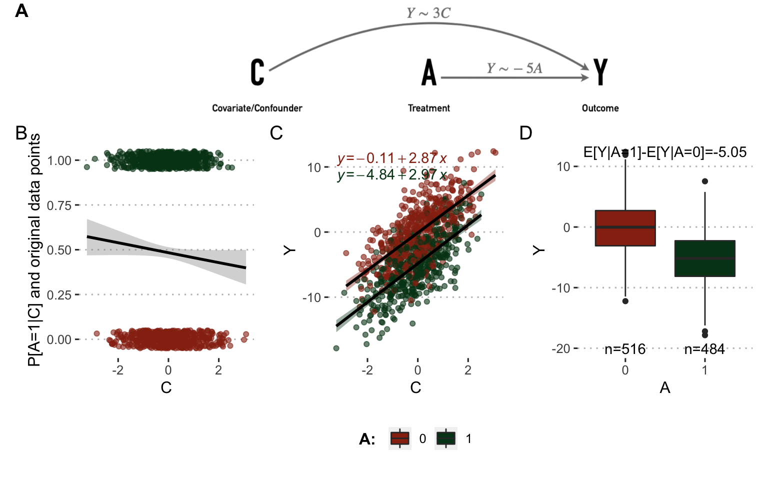
The situation can be illustrated with a simple simulated example involving a confounding variable \(C\) in addition to the treatment variable \(A\) and the outcome variable \(Y\). If \(Y\) represents tumor volume and \(A\) the treatment to be evaluated, \(C\) could be a biomarker of cancer agressiveness. 1000 patients have been simulated for all variables in two different settings represented in Figures 8.2 and 8.3. In the first case (Figure 8.2), the outcome \(Y\) is positively correlated to \(C\) (more agressive tumors have bigger volume) and decreased when \(A=1\) (treatment decreases tumor volume). \(C\) has no influence on \(A\). The causal relationships between the variables and the associated coefficients used to simulate data are summarized in the directed acyclic graphs (DAG) in Figure 8.2A. The observed relations between variables in simulated data are shown in Figure 8.2B, C and D. In particular, the theoretical influence of \(A\) on \(Y\) is recovered in the observed data since \(E[Y|A=1]-E[Y|A=0]=-5.05\)

Figure 8.2: Analysis on observed data without confounder. (A) Directed acyclic graphs with causal relations between variables and parameters used to simulate data. (B) Influence of \(C\) on \(A\) in observed simulated data. (C) Same with \(C\) and \(Y\). (D) Same with \(A\) and \(Y\).

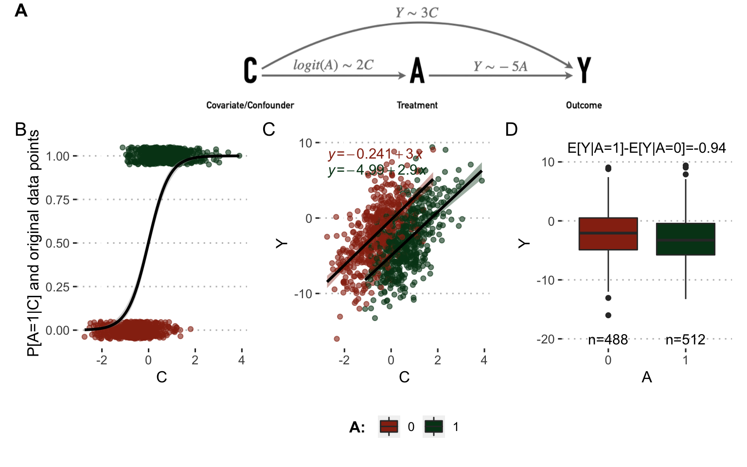
In the second case (Figure 8.3), \(C\) has an influence on \(Y\): the more aggressive the tumor, the more likely the patient is to be treated with the new drug. In this case the simultaneous influence of \(C\) on \(A\) and \(Y\) makes it a real confounder. The direct observation of the differences in outcomes between treated and untreated patients reveals only a small benefit of the new treatment which does not correspond to the underlying reality used in these simulations since the theoretical causal influence of \(A\) on \(Y\) remained the same as in the previous case. The confounding factor prevents the nature of the causal link between A and Y from being simply inferred.

Figure 8.3: Analysis on observed data with confounder. (A) Directed acyclic graphs with causal relations between variables and parameters used to simulate data. (B) Influence of \(C\) on \(A\) in observed simulated data. (C) Same with \(C\) and \(Y\). (D) Same with \(A\) and \(Y\).

8.2 Causal inference methods to leverage data

Despite these difficulties, some statistical methods have been developed to derive estimates with a causal interpretation from observational data, under precise assumptions. This work will focus on the potential outcomes framework (Rubin 1974). We will first describe briefly the fundamentals of this framework and different methods that are part of it.

8.2.1 Notations in potential outcomes framework

First of all, the notations used in this and the next chapter are defined as follows. We will use \(j=1,...,N\) to index the individuals in the population. \(A_j\) and \(Y_j\) correspond respectively to the actual treatment received by individual \(j\) and the outcome. In the most simple case, treatment takes values in \(\mathcal{A}=\{0, 1\}\), \(1\) denoting the treated patients and \(0\) the control ones. \(Y_j\) corresponds to the patient's response to treatment. In the case of cancer it may be a continuous value (e.g., size of tumor), a binary value (e.g., status or event indicator), or even a time-to-event (e.g., time to relapse or death). Only the first two cases will be discussed later. Finally, it is necessary to take into account the possible presence of confounders influencing both \(A\) and \(Y\) and denoted \(C_j\) for individual \(j\).

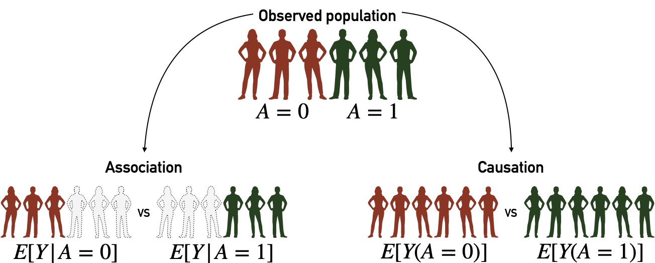
The potential outcomes framework is also described as counterfactual because it defines variables like \(Y_j(a)\) to denote the potential outcome of individual \(j\) in case he/she has been treated by \(A=a\) which may be different from what we observe if \(A_j\neq a\). This definition can be illustrated at the individual level, for patient \(j\), where \(A\) is the smoking status (\(1\) for smokers, \(0 otherwise\)) and \(Y\) is the outcome, e.g., cancer status at a given date. If patient \(j\) is a smoker then \(Y_j=Y_j(A=1)\). \(Y_j(A=0)\) would be the outcome if this same patient had not been a smoker, all other things being equal. This counterfactual outcome is therefore not observed in the data. These counterfactual variables make it possible to write the causal estimands. For instance, in this context, we can easily compute the difference in outcome between treated patients and control patients (Figure 8.4, left part): \(E[Y | A=1] - E[Y | A=0].\) However, this difference has no causal interpretation as it does not offer any guarantees as to the confounding factor, as an unbalanced distribution of \(C\) can induce biases. Thus we define another estimate: \(E[Y(1)] - E[Y(0)].\) In this case, we compare between two ideal cohorts (Figure 8.4, right part), one in which all patients have been treated (possibly contrary to the fact) and one in which all patients have been left in the control arm (once again, possibly contrary to the fact).

Figure 8.4: Association, causation and their associated cohorts. Association analyses are based on observed cohorts and conditional probabilities. Causation analyses are based on counterfactual variables and cohorts.

8.2.2 Identification of causal effects

The next question is whether it is possible to estimate the counterfactual variables \(Y(A)\) and under what conditions. The potential outcomes framework explicits assumptions of consistency, positivity and conditional exchangeability to estimate these counterfactual variables and therefore infer causal estimates from observational (non-randomized) data (Rubin 1974; Hernán and Robins 2020).

Consistency means that values of treatment under comparison represent well-defined interventions which themselves correspond to the treatments in the data: \(\textrm{if} \: A_j=a, \textrm{then} \: Y_j(a)=Y_j.\)

Exchangeability means that treated and control patients are exchangeable, i.e., if the treated patients had not been treated they would have had the same outcomes as the controls, and conversely. Since we usually observe some confounders we define conditional exchangeability to hold if cohorts are exchangeable for same values of confounding \(C\). Therefore conditional exchangeability will hold if there is no unmeasured confounding: \(Y(a) {\perp \!\!\! \perp}A | C.\)

Positivity assumption states that the probability of being administered a certain version of treatment conditional on \(C\) is greater than zero: \(\textrm{if} \: P[C=c] \neq 0, P[A=a | C=c] >0.\) Intuitively, this positivity condition is required to ensure that the defined counterfactual variables make sense and do not represent something that cannot exist.

Under these three assumptions, there are different methods and estimators available to evaluate causal effects from observational data. Two of them will be described and applied to the same example as above: the description of the example and the failure of the direct methods are recalled in Figure 8.5A and B and two causal inference methods are illustrated in Figure 8.5C, D and E.

8.2.2.1 Standardization or parametric g-formula

The first method is called standardization or parametric g-formula and it is the one that will be described in more detail in this chapter and the following one. It is based on the following equations:

\[\begin{equation*} \begin{aligned} E[Y(a)] & = \sum_{c} E[Y(a)|c] \times P[c] \\ & = \sum_{c} E[Y(a)|a,c] \times P[c] &&\text{ (exchangeability } Y(a) \perp \!\!\! \perp A | C \text{ )} \\ & = \sum_{c} E[Y|a,c] \times P[c] &&\text{ (consistency)} \end{aligned} \end{equation*}\]

Thus the average effect of treatment on the entire cohort can be written with standardized means:

\[\begin{equation} \begin{aligned} E[Y(A=1)] - & E[Y(A=0)] = \\ \sum_{c} \Big( & E[Y | A=1, C=c]-E[Y | A=0, C=c]\Big) \times P[C=c] \end{aligned} \end{equation}\]

Computationally, non-parametric estimation of \(E[Y | A=a, C=c]\) is usually out of reach. Thus, on real-world dataset, \(E[Y | A=a, C=c]\) is estimated through outcome modeling and explicit computation \(P[C=c]\) is replaced by its empirical estimate. The nature of the statistical model used will be specified in the various applications presented. In the simple example depicted in Figure 8.5A, a linear model of the outcome (\(Y\sim C+A\)) is fitted on observed data. This model is then used to infer \(E[Y | A=1, C=c]\) and \(E[Y | A=0, C=c]\) for each patient with covariate \(C=c\) (Figure 8.5C). By averaging these values over the whole cohort the confounding effect is corrected and the estimator is much closer to the true value \(-5\) than the naive estimates (Figure 8.5D and B).

Figure 8.5: Causal inference methods on a simple example. (A) Directed acyclic graphs with causal relations between variables and parameters used to simulate data. (B) Association between \(A\) and \(Y\) from observed data. (C) Some simulated samples/patients with their original variables (\(C\), \(A\) and \(Y\)), variables from outcome model (\(E[Y|A=0,c)]\), \(E[Y|A=1,c)]\)) and weights from treatment model (\(W^A\)). (D) Standardized causal effect of \(A\) on \(Y\) based on and outcome modeling. (E) IPW causal effect of \(A\) on \(Y\) based on weights derived from treatment modeling; in this panel weights are taken into account in boxplots and estimations.

8.2.2.2 Inverse probability weighting (IPW) and propensity scores

Based on the same counterfactual framework, it is possible to build another class of models, called marginal structural models (Robins, Hernan, and Brumback 2000), from which we derive estimators different from the standardized estimators called inverse-probability-of-treatment weighted (IPW) estimators (Cole and Hernán 2008). IP weighting is equivalent to creating a pseudo-population where the link between covariates and treatment is cancelled. In the case of binary treatment \(A \in {0 ,1}\), weights are defined for each patient as the inverse of the probability to have received the version of treatment he or she actually received, knowing his or her covariates:

\[W^A=\dfrac{1}{f[A|C]} \text{ with } f[a|c]=P[A=a|C=c],\]

\(f[a|c]\) being called the propensity score, i.e., the probability to have received the treatment \(A=a\), given the covariates \(C=c\). Again, propensity scores will be estimated in later examples using a parametric model. In this case with a binary treatment \(A\), a logistic treatment model is used (\(A\sim C\)) to derive the weights \(W^A\) (Figure 8.5C). Note that propensity scores are also useful for positivity investigations since values very close to \(0\) or \(1\) may indicate (quasi-)violations of positivity. Under the same hypothesis of exchangeability, positivity and consistency, we can derive the modified Horvitz-Thompson estimator (Horvitz and Thompson 1952; Hernán and Robins 2020):

\[\begin{equation} E[Y(a)]=\dfrac{\hat{E}[I(A=a)W^{A}Y]}{\hat{E}[I(A=a)W^A]}, \tag{8.1} \end{equation}\]

\(I\) being the indicator function, such as \(I(A=a)=1\) if \(A=a\) and \(I(A=a)=0\) if \(A\neq a\). Once again, this method brings estimates closer to the true causal effect by correcting for the influence of the confounder (Figure 8.5E).

8.2.2.3 Limitations and additional methods

These causal inference methods therefore allow to correct some biases due to observed confounders, at the cost of strong hypotheses that it is not possible to verify. The plausibility of these hypotheses, and therefore of the resulting estimates, requires a good knowledge of the context. Furthermore, the estimates are largely based on statical models of outcome or treatment. The correct specification of these models is therefore imperative to ensure unbiased causal estimates. In order to limit the risks of misspecification, some doubly robust approaches have also been developed. They require estimating both an outcome model and a treatment model, but the resulting estimates are consistent if at least one of the two models is correctly specified. One of these methodologies among others, called Targeted Maximum Likelihood Estimation (TMLE), will be mentioned in the next section and is detailed in appendix C.2.4.

In summary, evaluating the effect of a treatment requires isolating its impact from that of all confounding factors. This can be done in a randomized clinical trial designed for this purpose. However, there is a great amount of other data available that may not have been generated in this rigorous framework. It is nevertheless possible to draw causal interpretations from them, under certain hypotheses, thus offering insights for a posteriori statistical evaluation of specific therapeutic strategies.

Summary

In the process of evaluating a treatment, it is crucial to monitor the effect of confounding factors in order to identify the causal effect of the treatment and not spurious associations. This may involve randomized clinical trials specifically designed for this evaluation. In the case of observational data generated outside this framework, it is nevertheless possible to use causal inference methods to estimate, under certain conditions, the causal effect of the treatment.

References

Béal, Jonas, and Aurélien Latouche. 2020. “Causal Inference with Multiple Versions of Treatment and Application to Personalized Medicine.” ArXiv Preprint ArXiv:2005.12427.

Cole, Stephen R, and Miguel A Hernán. 2008. “Constructing Inverse Probability Weights for Marginal Structural Models.” American Journal of Epidemiology 168 (6). Oxford University Press: 656–64.

Hernán, MA, and JM Robins. 2020. “Causal Inference: What If.” Boca Raton: Chapman & Hill/CRC.

Horvitz, Daniel G, and Donovan J Thompson. 1952. “A Generalization of Sampling Without Replacement from a Finite Universe.” Journal of the American Statistical Association 47 (260). Taylor & Francis Group: 663–85.

Robins, James M, Miguel Angel Hernan, and Babette Brumback. 2000. “Marginal Structural Models and Causal Inference in Epidemiology.” LWW.

Rubin, Donald B. 1974. “Estimating Causal Effects of Treatments in Randomized and Nonrandomized Studies.” Journal of Educational Psychology 66 (5). American Psychological Association: 688.